The Value of Optical-Fiber Isolated Probes in EV Traction Drives: The Price of a Bad Measurement Can Be an Inverter Leg
Release Time:2026-11-09
With 800 V platforms and SiC devices going into volume production, DC bus voltages have climbed sharply and switching speeds are an order of magnitude faster — and the safety margins in power-circuit design keep shrinking. The design, calibration, and validation of inverter legs all depend heavily on waveform capture at high-voltage floating nodes; once a waveform measurement is distorted, destroyed bridge-leg devices are never far away.
Today's mainstream probing solutions fall into two camps. High-voltage differential probes cost less, but the measurement loop remains electrically coupled to the circuit under test. Optical-fiber isolated probes convert the signal to light and carry it over fiber — a higher purchase price, but a far lower risk of wrecking bench equipment, solid support for precise calibration of dead time and other critical parameters, and less spend on redundant components. Accounting for the gains across equipment damage, development time, material cost, and vehicle-level energy consumption, the payback period of an optical-fiber isolated probe typically comes in under three months.
1. Measurement Challenges in Traction Drive Systems
Traction-drive development has to cover power-device reliability assessment, switching-timing verification, and analysis of how common-mode interference affects bearings — all of it resting on nanosecond-scale transient signals. And the test environment throws up three hard obstacles:
l Floating measurement points: the high-side gate reference potential swings dynamically across the 0–800 V range;
l Steep switching edges: SiC devices reach dv/dt of tens of volts per nanosecond, and insufficient probe bandwidth simply flattens the voltage spikes;
l Multi-channel coupled interference: with several channels measuring at once, common-ground coupling adds noise that confuses signal interpretation.
A high-voltage differential probe relies on a front-end divider network for common-mode rejection, and that performance decays quickly as frequency rises: roughly 80 dB of CMRR at DC, down to only about 30 dB at 100 MHz. On an 800 V bus, the 100 MHz band alone can inject a spurious common-mode voltage of about 25 V. The turn-on threshold of a SiC MOSFET is only 2–3 V — a phantom voltage of that size is easily enough to falsely turn the device on, with all the misjudgment risk that implies.
An optical-fiber isolated probe converts the measured voltage into light and carries it over fiber, cutting off the common-mode conduction path entirely. With input capacitance as low as 1 pF and a CMRR of 128 dB at 100 MHz, the residual interference is only about 0.3 mV — far below the 2–3 V turn-on threshold of SiC devices, ruling out false turn-on.
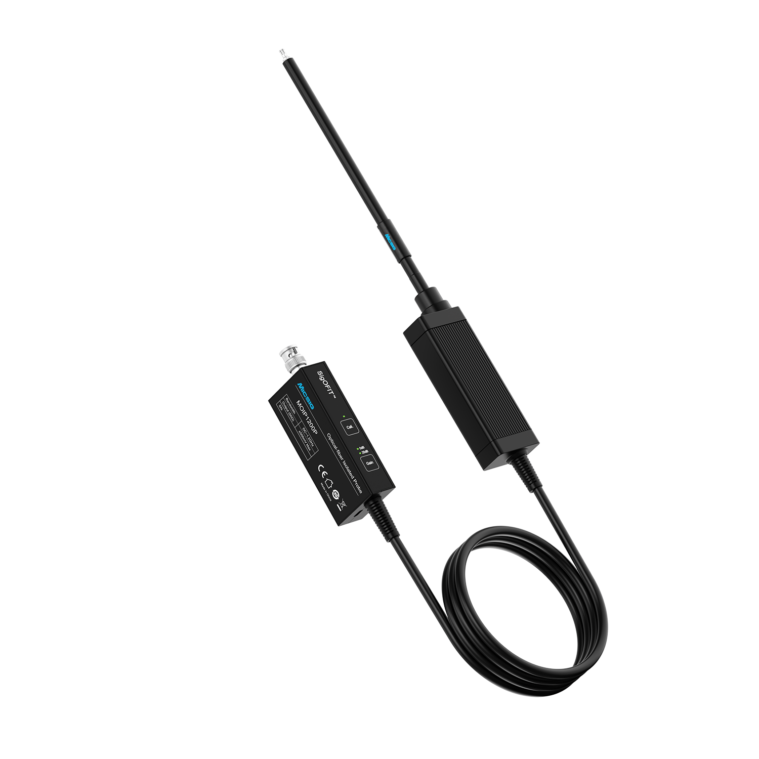
SigOFIT™ MOIP series optical-fiber isolated probes (image source: Micsig official website)
Micsig SigOFIT™ MOIP selection guideline: for gate timing and bus ripple measurements, a 350–500 MHz bandwidth is the right choice; for turn-off overshoot, bridge-leg crosstalk, and common-mode dv/dt analysis, go with 1 GHz or above.
2. Three Typical Risk Points in Bench Testing
During bench debugging, many project stalls trace back not to hardware design flaws but to distorted measurement data leading engineers astray. The table below compares high-voltage differential probes with the Micsig SigOFIT™ MOIP optical-fiber isolated probe — and what a wrong call actually costs.
Decision point | High-voltage differential probe | Micsig SigOFIT™ MOIP | Cost of a misjudgment |
Turn-off overshoot / only a few hundred volts of margin on 800 V platforms | Edges smoothed out and spike readings biased low — the steeper the edge, the lower the reading | Rise time ≤350 ps / overshoot captured in full | The power device gets selected one voltage class too low; the bench looks fine, but the part may break down once installed in the vehicle |
Bridge-leg crosstalk / low-side Vgs rise, judged against the 2–3 V threshold | Common-mode residue rides on Vgs / high-side and low-side timing cannot be compared directly | Rejection that does not collapse with frequency / independent channels, timing directly comparable | Dead time gets padded as a safety net; 100 ns of extra dead time costs both efficiency and NVH |
Common-mode dv/dt / shaft voltage and bearing electrical erosion | Edges smoothed / both dv/dt and common-mode current read low | Edges faithfully reproduced / dv/dt quantifiable | Countermeasures get bolted on wholesale; BOM and process costs both rise, and there is still no evidence to show for it |
Notes: High-voltage differential probe figures reflect typical mainstream products on the market; optical-fiber isolated probe figures follow the published specifications of the Micsig MOIP series; “cost of a misjudgment” describes the practical consequences of carrying the design forward on distorted data from the original high-voltage differential probe.
3. The Value Case: Investment, Return, and Payback
Moving from high-voltage differential probes to optical-fiber isolated probes adds roughly ¥40,000–80,000 to the procurement bill. The return spans four dimensions — bench hardware damage, calibration iteration labor, redundant-countermeasure material cost, and vehicle-level energy savings. Modeled for different types of businesses, avoided bench-device damage alone recovers the added investment on a passenger-car program within the year.
Return dimension | Passenger-car traction | Commercial vehicle / construction machinery | High-performance in-house programs |
Typical platform | 800 V SiC | 1000 V+ high power | 800 V + SiC / GaN |
Added investment | 6 channels / added investment ≈ ¥60,000 | 4 channels / added investment ≈ ¥40,000 | 8 channels / added investment ≈ ¥80,000 |
A · Avoided bench hardware damage (device breakdown, shoot-through faults) | 2 × ¥35,000 / ¥70,000 | 1 × ¥50,000 / ¥50,000 | 2 × ¥60,000 / ¥120,000 |
B · Calibration iteration labor saved | 6 × 1 × 2 × ¥3,500 / ¥42,000 | 4 × 1.5 × 2 × ¥3,500 / ¥42,000 | 3 × 3 × 3 × ¥4,000 / ¥108,000 |
C · Redundant-countermeasure BOM savings | ¥2 × 60,000 / ¥120,000 | ¥5 × 8,000 / ¥40,000 | ¥2 × 30,000 / ¥60,000 |
D · Vehicle energy savings / 25% attribution | 540,000 kWh / ¥135,000 | 1,020,000 kWh / ¥256,000 | 270,000 kWh / ¥67,500 |
Total annual benefit | ≈ ¥367,000 | ≈ ¥388,000 | ≈ ¥356,000 |
Overall payback period (A+B+C+D, including energy savings) | ≈ 2.0 months | ≈ 1.2 months | ≈ 2.7 months |
Company-side payback (A+B+C, excluding energy savings) | 3.1 months | 3.6 months | 3.3 months |
1. A covers power modules, equipment damage, and downtime/troubleshooting labor; C applies only to all-new platform programs, where the cost is amortized across the full model line.
2. D follows industry rules of thumb: gate measurement error tightened from ±3% to ±0.3%, allowing dead time to shrink by 50 ns and switching losses to drop by 0.4%, lifting vehicle efficiency from 97.5% to 97.9%; at 15,000 km per year, that is roughly 9 kWh saved per vehicle. The model uses ¥1/kWh and attributes 25% of the gain to measurement accuracy; the direct beneficiary of the energy savings is the end user, while the OEM's equivalent benefit shows up as a smaller battery for the same range.
3. All figures are industry-typical modeled values; companies should recalculate with their own business data.
4. Closing Thoughts
The key metrics of a traction-drive product — device safety margin, dead-time parameters, and vehicle-level energy efficiency — are, to a large extent, determined by how true the bench-test waveforms are.
For 400 V and below silicon IGBT platforms, high-voltage differential probes still offer good value for money. But once a program steps up to an 800 V platform with SiC devices, differential probes readily deliver distorted waveforms, and calibration starts iterating endlessly. So the value of a probe should not be judged on purchase price alone — equipment damage, development iterations, and vehicle-level performance carry hidden costs that matter far more. Viewed across the production line and the full project life cycle, the payback period of an optical-fiber isolated probe is typically under three months.
To evaluate probe selection for your specific topology and operating conditions, or to arrange a hands-on evaluation with a demo unit, contact Micsig at sales@micsig.com or your local authorized distributor.
Data Notes
Product parameters cited in this article are drawn from public technical documentation of the Micsig SigOFIT™ MOIP series; refer to the latest product datasheets on the official website. Common-mode residue and edge-fidelity values are engineering estimates for typical operating conditions; the energy-loss chain in Section 3 uses industry experience values to indicate order of magnitude.
The application scenarios listed summarize common operating conditions in traction-drive development. The benefit calculations are modeled for the three business types using industry-typical values; actual returns vary with product positioning, power level, and team configuration — base your own decisions on your own measured data.