The Value of Optically Isolated Probes in GaN/SiC Device Design: Pay for the Architecture, Save on Misjudgment

Wide-bandgap (WBG) devices such as GaN and SiC are becoming the mainstream choice for high-efficiency power supplies and electric drives. As switching speeds climb, so does the difficulty of measuring them. For high-voltage floating nodes, engineers typically choose between two probe families: high-voltage differential probes and optically isolated probes. The latter offers a far wider performance envelope, at a noticeably higher purchase price—which is exactly the trade-off weighed most often at selection time.

Under wide-bandgap operating conditions, however, the real question is not “how much more does it cost?” but “is the measurement still accurate enough?”—the cost of a misjudgment is often a board respin, or worse, a destroyed device. This article proceeds in three steps: first, where the measurement difficulty lies; then, the cost of misjudgment broken down by scenario; and finally, a payback calculation showing how quickly the price premium comes back.

1. What Makes Wide-Bandgap Measurements So Hard

The difficulty lies in the operating conditions themselves. The effective swing of the high-side V_GS is typically only a few volts up to twenty—commonly 0–6 V for GaN and −4 V to +18 V for SiC—while its reference point, the switch node, is simultaneously subjected to common-mode transitions of several hundred volts at slew rates of tens of V/ns. The measurement front end must therefore resolve a differential signal of a few volts—even a few hundred millivolts—riding on a common-mode background of hundreds of volts, while keeping up with sub-nanosecond switching edges.

Translated into three probe requirements, any single one of them can make or break the measurement.

First, bandwidth. Bandwidth determines the probe's own rise time: BW × t_r ≈ 0.35, so 350 MHz corresponds to roughly 1 ns. The edge displayed on screen has a rise time equal to the root-sum-square of probe and signal: t_r(total) = √(t_r(probe)² + t_r(signal)²). The slower the probe, the further what you see deviates from the true edge. To faithfully capture sub-nanosecond switching edges, at least 350 MHz is required—ideally ≥ 1 GHz.

Second, common-mode rejection ratio (CMRR). Every switching-node transition is hundreds of volts, and whatever common-mode residue remains lands directly on top of a gate signal of just a few volts. If CMRR is insufficient, the signal is drowned in common-mode noise before it ever reaches the oscilloscope—past that point, accuracy is moot.

Third, input capacitance. Once connected, a probe is no longer a bystander: a few picofarads shunted onto a high-impedance node alter the very waveform being measured, together with the source impedance and lead inductance.

For high-voltage differential probes, these three parameters are mutually constraining—pushing any one of them forward comes at the expense of cost, noise, or voltage rating. Mainstream models therefore generally plateau at the hundred-megahertz level, with common-mode voltage ratings around 1.5 kV. Micsig's SigOFIT™ optically isolated probes take a fundamentally different route—an “optoelectronic conversion + fiber-optic isolation” architecture that sidesteps this constraint altogether: the MOIP series pushes bandwidth to 1.2 GHz and common-mode voltage to 85 kV_pk, with a DC CMRR of 180 dB across the lineup—still 106 dB at 1.2 GHz.

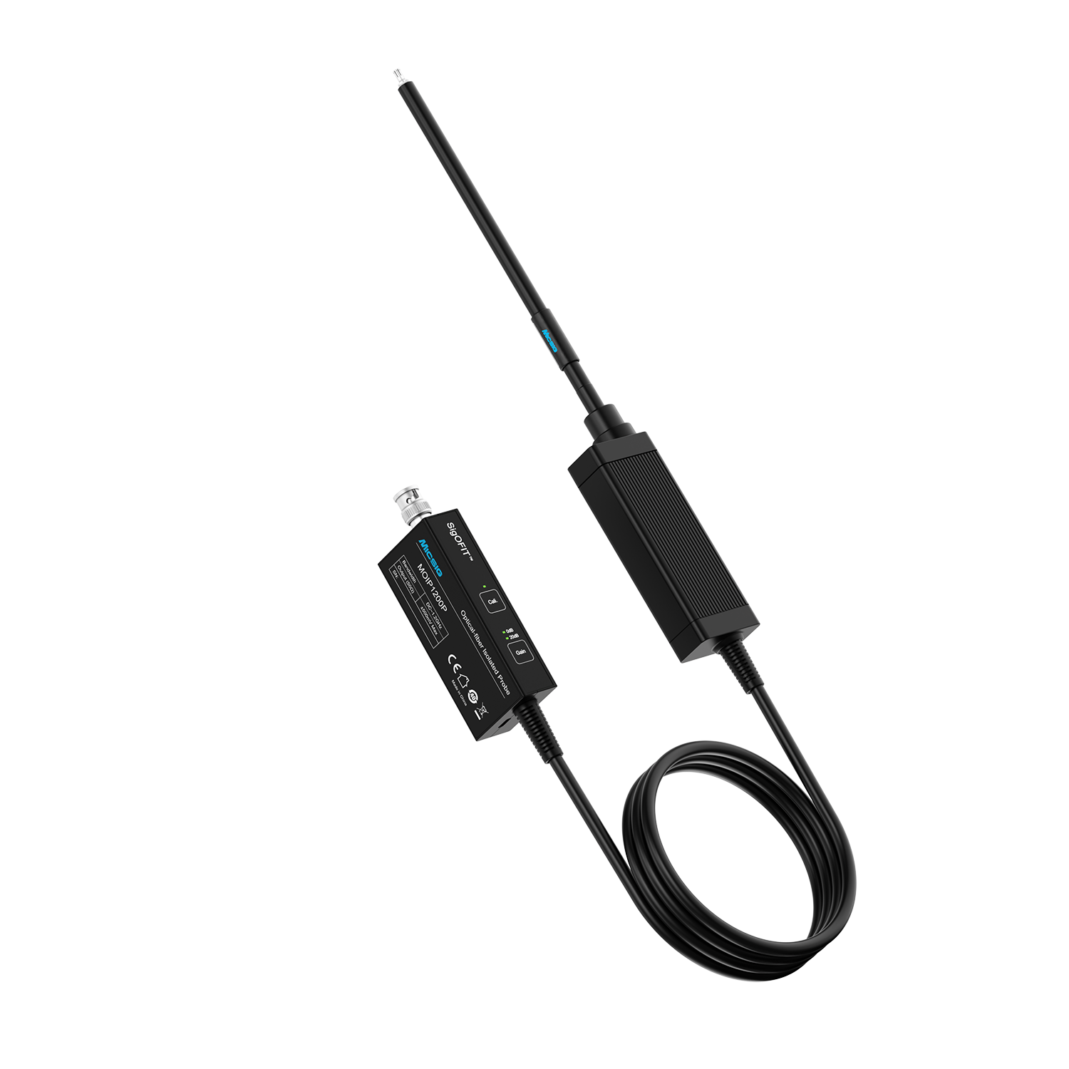
SigOFIT™ MOIP series optically isolated probes

Consider just one figure: the common-mode residue from a 500 V common-mode step at 100 MHz. A high-voltage differential probe leaves roughly 15.8 V; an optically isolated probe, about 0.2 mV—nearly five orders of magnitude apart. This is no longer higher versus lower accuracy; it is a difference in orders of magnitude. On the bench it boils down to one question: is this waveform even fit to be interpreted?

2. Value Comparison in Typical Test Scenarios

Dynamic measurements appear at many points in GaN/SiC device design. The three scenarios below place the harshest demands on the measurement front end; the same logic applies everywhere else.

Notes: ① Differential-probe figures reflect performance levels commonly published in industry technical literature; optically isolated probe figures follow the published specifications of the Micsig MOIP series. ② “Cost of misjudgment” refers to the cost caused by misjudgment due to waveform distortion when continuing to use a differential probe.

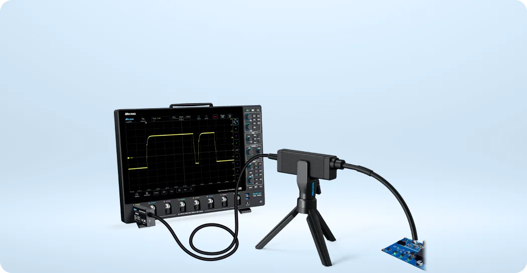
SigOFIT™ probe paired with a high-resolution oscilloscope for a double-pulse test

3. The Value Payback: Three Independent Channels—Count the Ones You Use

The value of the three judgment points above ultimately flows through three independent channels: no more destroyed devices, no project rework, and fewer prototype respins. Here we turn that value into numbers. Assume an existing 4-channel oscilloscope in which the high-voltage differential probes are replaced with Micsig SigOFIT™ optically isolated probes (MOIP series); take only the tests you actually run. The incremental outlay is simply the price difference between the two, while the savings are the very real costs of destroyed devices, rework, and board respins. The calculation, itemized by test type actually performed, is as follows:

Basis of calculation: A assumes 2 SiC module failures per year at ¥20,000 each (samples, instrument time, and labor included); B assumes 4 projects, each shortening its bring-up schedule by 2 weeks, staffed with 2 engineers at ¥3,000 per engineer-week; C assumes that cutting the measurement misjudgment rate from 3% to 0.2% eliminates about one redundant board respin per year across 4 projects, at ¥18,000 per respin. The three channels are independent—count only the ones that match the tests you actually run; not every team will realize all of them. Even at a conservative 50% haircut, the payback period never exceeds two years, and the shortest case still lands within six months.

The figures above are based on an industry-typical-value model; we recommend plugging in your team's own data to verify.

4. Closing Thoughts

The performance of a wide-bandgap device often comes down to details on a nanosecond-scale switching edge. Whether that edge is captured faithfully determines whether everything that follows stands on measured evidence—or remains speculation without it.

So back to the opening question: the right thing to ask about this investment is not “how much more does it cost?” but “is it still accurate enough?”. If your flagship products are still silicon-based with ample switching-edge margin, your current setup is good enough. But once you push switching speeds into the sub-nanosecond range, the measurement front end becomes the ceiling of your design judgment—whatever magnitude it stops at is where your design stops.

The SigOFIT™ MOIP series was built for exactly this: 85 kV_pk common-mode voltage, 1 pF input capacitance, and 180 dB CMRR integrated into a single optically isolated probe, so that high-speed switching edges are reproduced faithfully—and measurement accuracy no longer caps design judgment.

For selection support on your specific devices and test plan, or to arrange hands-on evaluation with a demo unit, contact Micsig at sales@micsig.com or your local authorized distributor.

Data Notes

Product specifications cited in this article are subject to the latest Micsig datasheets.

The benefit calculations are model-based estimates using industry-typical values; actual results vary with device type, test scale, team setup, and operating conditions—defer to your own measured data.